Unicursal mazes and "Cavern" mazes

Mazes: Generalities

There are many kinds of mazes, and many ways to classify them. Some mazes have loops, but most don't. Most mazes have no inaccessible areas, and are usually drawn on a square grid. The mazes that meet the requirements of having no inaccessible areas (i.e. all passages are connected) and no loops are called perfect mazes.

Mazes are intimately related to graph theory. The most common type of maze can be represented by an undirected graph (but there are also many other types of mazes which need a directed graph to be represented, including arrow mazes and "mazes with rules"), it has no loops (and is therefore a tree) and has every room (vertex) connected to all others. In graph theory terms, that's exactly what a spanning tree is. In maze jargon, that's called a perfect maze. In other words, the terms perfect maze and spanning tree are equivalent, in their respective contexts.

Perfect mazes are the most common type because they meet two desirable properties. First, since there are no loops, the solution (the route from a given vertex labeled "start" to another given vertex labeled "end") is unique, not counting backtracking from a dead end. Second, since they don't have any unreachable areas, they make the most use of the available space (usually a rectangle). Actually, I personally think that the no loop condition makes them kind of boring, because it makes them trivial to solve (by wall-following). But this article is not about solving difficulty. It has more to do with aesthetics and graph theory.

Representing a maze

For a compact representation, two-dimensional mazes are usually represented in a bitmap by having the vertices (rooms, in maze jargon) at odd-numbered rows and columns (assuming the first row and column is 0, as we're usually dealing with bitmap coordinates), then having some cells that are always walls and some cells that may or may not be walls, depending on whether the corresponding graph has an edge at that position (passage) or not (wall).

12×12 grid graph as is commonly represented in a compact way in a cell grid. The white cells are always walls, the black cells are always empty, and the blue cells represent pixels that are to be turned into white or black to give shape to the maze. In the corresponding grid graph, the blue cells represent the edges, the black cells represent the vertices, and the white cells are empty spaces. The cross-faded image depicts the graph itself for comparison. A perfect maze is a spanning tree of that graph.

There's another common way of depicting mazes, using squares with missing sides for the rooms, where the present sides are the walls. But we're not interested in it now.

Observe that a maze constructed using that kind of template will always have the passages and the walls one pixel wide, and that there won't be any walls or passages touching only diagonally. In other words, there are three 2×2 patterns that no 2×2 subset of the bitmap will match: all walls, all passages, and a checkerboard pattern. That's guaranteed by the fact that every single 2×2 subset of the bitmap will always have at least one black cell in one corner (the vertex) and one white cell in the opposite corner (the empty space), regardless of the values of the other two.

The top row shows the 2×2 patterns that will never appear in any 2×2 subset of the maze image (2×2 wall, 2×2 passage, and 2×2 checkerboard in its two variants). The rest of the patterns can appear anywhere.

Unicursal mazes

There is a kind of maze that is... well, hardly a maze actually. It's called a unicursal maze, which is a maze with no dead ends and no loops. That's right: it is just a single path that can be followed from the beginning to the end without finding any intersections in the way. Sounds dull? Keep reading!

A unicursal maze is not necessarily perfect: it may not meet the condition of going through all possible rooms. Obviously, a perfect unicursal maze is a Hamiltonian path in graph theory terms: a path that goes from one point to another, visiting every vertex in the graph exactly once. This equivalence has at least two major implications. First, we can't always have a perfect unicursal maze with any arbitrary starting point and any arbitrary ending point, even in a rectangular grid graph. Second, creating a perfect unicursal maze with chosen endpoints is not a trivial task, if possible at all. Turns out unicursal mazes aren't that dull, after all!

Let's quickly review the conditions that the endpoints must meet, in order to be possible to have a perfect unicursal maze. The maze dimensions should both be 4 or more, or 3×(odd number ≥ 3), to exclude some special cases that are hard to handle, as some have a solution and some don't. The rest of the conditions depend on whether the associated rectangular grid graph has an odd number or an even number of vertices. If the number is even, then the only condition is that the sum of row + column of the starting point and the sum of row + column of the ending point must have different parity. If the number of vertices is odd, the parity of the endpoints must be the same, but there is another condition: they also need to have the same parity as the vertices in the corners. There's a demonstration in [1]. If a rectangular grid graph with the required dimensions meets these conditions, it's guaranteed that at least one Hamiltonian path exists between both. If not, it's guaranteed that none exists. In other words, the conditions are necessary and sufficient for those grid graphs. The conditions for 2×n, 1×n, and 3×(even number) are too complex for this quick synopsis; take a look at the paper if interested. Of course, what is said for m×n is valid also for n×m.

Creating perfect unicursal mazes

So, how to create a random perfect unicursal maze? One possible way is to create a Hamiltonian cycle and break it, using the split points as start and end. This obviously reduces the problem to creating a Hamiltonian cycle. A trick used to create such a cycle consists of applying the following concept: create a regular maze, and then add a wall in the middle of each passage.

Perfect maze (left) and unicursal loop resulting from it (right). The loop can be broken at any edge next to one of the exterior walls and parallel to it (marked in red), to give a unicursal maze that starts and ends at a border.

But that method creates unicursal mazes with a very clear pattern: every single-step edge (in the sense of not turning while walking it) is preceded and followed by two-or-more-steps edges. That's certainly not what one expects from a random Hamiltonian path with any signs of uniformity. It is only able to generate a small subset of the possible Hamiltonian paths. Even if the algorithm is modified to enable arbitrary starting and ending points (arbitrary among the ones that meet the necessary conditions for a Hamiltonian path to be possible), that problem will still exist with that method. Is there an algorithm that allows for the whole range of possibilities of Hamiltonian paths?

Fortunately, yes. Not exactly uniformly distributed, but not too far either. It's capable of generating every possible Hamiltonian path, with a probability distribution that is empirically not distinguishable from a uniform distribution. The paper describing the method and the empirical results is [2], and to the surprise of many, including me, it's about polymers. Yes, the molecules. It turns out that random Hamiltonian paths have an important role in the field of polymer chemistry. Live and learn.

Let me outline the method. Start with a non-random, easy to build Hamiltonian path, consisting of going in zig-zag from one end of the top row to one end of the bottom row. Actually, the starting pattern does not matter much, but that's an easy way to build one in a rectangular grid graph. Then repeatedly apply a transformation of that path that they call "backbite", using one of the two endpoints at random every time. A backbite transforms a Hamiltonian path into a different one that is also Hamiltonian, and it consists of the following: from one endpoint, choose a neighbouring vertex at random that is not connected to the current one. If the chosen vertex turned out to be the opposite endpoint, add an edge to it and remove the edge that it was connected to originally. If it is not the opposite endpoint, add an edge that connects to it. That will create a loop for sure, and the destination vertex will now have three edges. One of them will be the one just created and another one will lead to the opposite endpoint. The third edge loops back to itself. Remove it to obtain a graph that is again a Hamiltonian path, but with a different endpoint. That's the backbite move.

Backbite move on a 3×3 graph. Starting with a Hamiltonian path (1), choose an endpoint (red in this case) and a neighbouring vertex at random that is not connected to that endpoint. In this case there's only one, so an edge is added that connects to it (2, in green). The target vertex (3, in green) has two other edges apart from the one just added: one leading to the opposite end (blue) and another looping to ourselves (red). Complete the move by removing the latter, resulting in another Hamiltonian path (4) with a new endpoint (in red).

By repeating the backbite move enough times, the authors of the paper show how the resulting path is approximately uniformly distributed, according to several criteria.

This method has two main disadvantages. First, it's not easy to determine when to stop, and given that the backbite move is relatively expensive, making many more moves than necessary to be in the safe side is slow. Second, both endpoints end up at unknown locations.

Another method that also uses the backbite move, is to perform a (non-overlapping) random walk starting from one chosen point, and when it is not possible to go on because all neighbours are already visited, perform one single backbite (on the blocked end only) and then try again the random walk. (One rare exceptional case: if the backbite move leads to the original endpoint, switch endpoints, as we want one of them to be at a fixed location.) Repeat the process indefinitely. Eventually, if the starting endpoint was chosen so that it obeys the conditions, we will obtain a Hamiltonian path with a known start and a random end. A series of backbites on that end can help us now place the endpoint at a desired location (always chosen by the rules). That path may not be uniform, but visually it's hard to tell the difference. The main advantage is that it has better guarantees that all edges are visited and randomized. With the other method, some areas may remain unvisited by the repeated backbite and therefore left in their original state.

12×12 perfect unicursal maze (Hamiltonian path) and 12×12 perfect unicursal loop (Hamiltonian cycle) created with the technique described.

Cavern mazes

It is possible to construct mazes that do not obey the pattern in the first figure, that is, mazes whose walls are not aligned in a grid of the kind described. Every pixel would be a vertex, and every pair of passage pixels vertically or horizontally adjacent would be connected by an edge. These mazes are no longer spanning trees of a grid graph, as there are many disconnected vertices (one per wall pixel), but compared to the perfect mazes we've seen so far, they share the characteristics of having no isolated connected areas or loops and being trees, so we'll extend the concept of "perfect maze" to also include those that have isolated vertices, for discussion purposes. Walter D. Pullen [3] calls those "cavern" mazes, and we're using the same term here for lack of any others. There are several ways to construct them. Usually, not all the 2×2 exclusion patterns mentioned earlier are absent in the mazes created this way; most of the times, there are 2×2 checkerboards and/or 2×2 walls and/or 2×2 passages at some points.

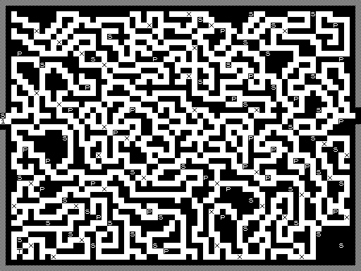
Let's take as an example the maze generated by the good old ZX81 program Mazogs. Mazogs is a game in which you are in a 62×46 dungeon or cavern, with passages organized like a maze, and your aim is to search for the hidden treasure in the cavern with the help of the prisoners scattered around the maze, avoiding to run into a Mazog (or if you do, you better hava a sword with you; swords are also scattered around), then return to the entrance. It had a very well done atmosphere at the time (1982). You really felt like it was a cavern with dark passages. And part of the ambience was provided by the fact that the maze did not look too geometric, but more like random passages in a real cavern. When its successor, Maziacs, came for the ZX Spectrum, I was disappointed because it lost that feeling due to the change in the style of maze: it was of the kind described at the beginning, and thus no longer a cavern maze. It lost the sensation of being dungeon-ish, and felt more geometric due to the longer passages. The added complications didn't really improve the gameplay in my opinion. But the point here is that the shape of the maze did have an important role in the overall feeling of the game. The name "cavern" is well deserved.

One characteristic of the mazes created by Mazogs is that it could easily create 2×2 checkerboard blocks, as well as wall-only 2×2 blocks, but never 2×2 passage blocks.

Example of a maze generated by Mazogs. "1" is the player (at the starting point in this case), "T" is the treasure, "X" are mazogs, "S" are swords, "P" are prisoners that reveal the solution when run into. The generation method is a "hunt and kill" variant, where the hunt phase is random rather than sequential, and the kill phase considers whether there are passages next to the candidate to be carved, and carves one cell at a time. The program has a time limit for generating the maze, and a minimal amount of passages for it to be considered valid. If that minimum is not met, the algorithm restarts.

Pullen has a program for Windows, called Daedalus, that is able to generate cavern mazes with no 2×2 checkerboards, and you can decide whether you want no 2×2 passages, or no 2×2 walls, but not both (unless you're really, really lucky and get one by chance). Daedalus runs under Wine although with some flicker, at least in my system.

Cavern mazes generated by Daedalus. Neither has a 2×2 checkerboard pattern (passages touching diagonally). The one on the left was generated by passage carving, and has 2×2 walls. The one on the right was generated by wall adding, and has 2×2 passages. The scarceness of walls that start at the border in the right image (there are long passages that run throughout most of the side walls) is typical in this program when generating a cavern maze this way.

Is it possible to generate cavern mazes that are guaranteed to meet all three criteria (no 2×2 checkerboard, walls, or passages)? The answer is of course yes, but here comes the funny part: the problem of generating such a maze is equivalent to generating a Hamiltonian cycle in a grid graph.

How's that possible? Note the frontier between the wall and the passage, imagining it as a graph. Having a 2×2 checkerboard pattern somewhere, would mean we have a vertex with four edges converging to it, but that's excluded. Having a 2×2 wall or passage would mean that one vertex has no edges leading to it, but these patterns are also excluded. Every other combination of 2×2 cells has a frontier that has exactly 2 edges, therefore every vertex of that graph has exactly 2 edges connecting it. That means that it must form loops that pass through every vertex in the graph. But since it encloses the passage area, which is (by definition of a perfect maze) one single area, it can't form more than one loop. Consequently, it is one single loop that passes through all vertices, i.e. a Hamiltonian cycle. Effectively, this process is equivalent to doing the reverse operation to adding a wall in between the passages, that we mentioned as one method of creating a perfect unicursal maze. In this case, since the loop encloses a wall, we remove it.

This is a 13×13 cavern maze generated by using the 12×12 Hamiltonian cycle shown earlier as the frontier of the walls. It has no 2×2 checkerboard, wall or passage block.

Equivalent graph for the cavern maze above. The red dots represent unconnected vertices.

65×65 cavern maze generated from a 64×64 Hamiltonian cycle.

Cavern mazes generated this way look quite nice in my opinion. Of course that's a question of taste, so YMMV. One problem they have, however, is that, just like with uniform random spanning trees, they tend to have lots of short passages, instead of being primarily made of long winding ones that would play a better role in confusing the player. So far I've found no solution for this, but a promising idea is to start by building a cavern maze with the desired properties except for the 2×2 wall blocks, then modify it to make these blocks disappear. It's not easy to do the latter; it's impossible to make just one single block disappear (other than by creating a 2×2 passage block, which obviously isn't the desired result). However, it's possible to use two such blocks so that with local modifications in between, they cancel each other. So far I haven't figured out an algorithm that is able to do that, but I've been able to do it by hand. Not all pairs of 2×2 blocks can be cancelled this way; they have to be of opposite parity (the parity of such a block is the parity of its central vertex, when seen as the frontier graph, obtained from the sum of its row and column, modulo 2).

Example of a section of a maze that has two 2×2 wall blocks (left) with the parity of the vertices marked with green and yellow dots, showing that the blocks have different parity. When that's the case, it's possible to modify some pixels in such a way that the blocks cancel each other and disappear. The image on the right shows one of many possible ways to do it.

Is there a move, similar to the backbite, that allows displacing an isolated vertex of a certain parity to another position without changing any characteristics of the graph? If so, joining vertices of opposite parity should not be difficult: when they are next to each other, usually one pixel change suffices to cancel both. I'd be interested in knowing about an algorithm that can do that.

Update (2017-04-03)

I forgot to mention that in order for a rectangular grid graph to have a Hamiltonian cycle, it must have an even number of vertices, therefore rectangles with an odd number of vertices on each side can't have one. The reason should be obvious when considering that any Hamiltonian cycle can be obtained from a Hamiltonian path that has the two endpoints adjacent, then adding an edge between them to close the loop. Adjacent vertices always have opposite parity, and when the number of vertices is odd, they must have the same parity, therefore they can't be adjacent, therefore they can't form a loop.

References

[1] Alon Itai, Christos H. Papadimitriou and Jayme Luiz Szwarcfiter, Hamilton paths in grid graphs. SIAM Journal of Computing, 11(4):676—686, 1982.
[2] Richard Oberdorf, Allison Ferguson, Jesper L. Jacobsen and Jané Kondev: Secondary Structures in Long Compact Polymers (2008) (preprint).
[3] http://www.astrolog.org/labyrnth/daedalus/daedalus.htm